Fractal Find : Explore Fractal and Quantum Variations

CHAPTER 3
Polar Coordinate Unit Circle Variations

Basic Julia Set with Pseudocode

for (int i = 0; i ≤ 500; i++)
{
	for (int j = 0; j ≤ 500; j++)
	{
		xs = 0.0;
		ys = 0.0;
		x = -2.5 + (i / 100.0);
		y = -2.5 + (j / 100.0);
		k = 0;
		do
		{
			k = k + 1;
			xnew = x*x - y*y + xs;
			ynew = 2.0*x*y + ys;
			x = xnew;
			y = ynew;
		} while ((k ≤ kmax) && (x*x + y*y ≤ 6.25));
		PlotPixel(i, j, color);
	}
}

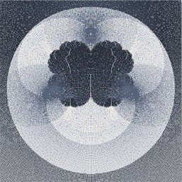
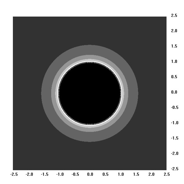
Unit Circle using Cartesian Coordinate Points

When x² + y² < 1.0, points collapse to (0.0, 0.0)
When x² + y² > 1.0, points increase in magnitude with each iteration.
When x² + y² = 1.0, points are on the unit circle and remain on the unit circle for subsequent iterations. However, due to iterative round-off errors in Cartesian coordinates, unit circle points either converge to (0.0, 0.0) or increase with each iteration. The unit circle exists, but iterative round-off prevents acccurate representation in Cartesian coordinates.

Note:
In these figures, (1.0, 0.0) is a final value and is on the unit circle.
The symbol "+" designates points when count exceeds maximum value as single pixels are difficult to view.

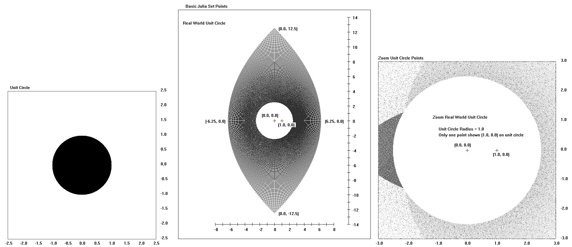
Julia Cartesian	Build: (f(x,y), g(x,y), (xs,ys))	Escape: h(x,y)>value	Plot
Basic Julia Set	(x² - y², 2.0xy), (0.0, 0.0)	x² + y² > 6.25	Pixel
Unit Circle	(x² - y², 2.0xy), (0.0, 0.0)	x² + y² > 6.25	Pixel
Julia Set Points	(x² - y², 2.0xy), (0.0, 0.0)	x² + y² > 6.25	Point
Unit Circle Points	(x² - y², 2.0xy), (0.0, 0.0)	x² + y² > 6.25	Point

Unit Circle in Polar Coordinates with Pseudocode

for (int i = 0; i ≤ 44; i++)
{
	for (k = 1; k ≤ 8; k++)
	{
		θ = 2.0*θ;
		x = cos(θ);
		y = sin(θ);
	}
	PlotPoint(x, y, color);
}

In Cartesian coordinates:
x = x² - y²
y = 2.0*x*y

In polar coordinates:
cos(2.0*θ) = cos(θ)² - sin(θ)²
sin(2.0*θ) = 2.0*cos(θ)*sin(θ)

Rewriting the equations:
x = cos(2.0*θ) where x is the real portion of the expression.
y = sin(2.0*θ) where y is the imaginary portion of the expression.

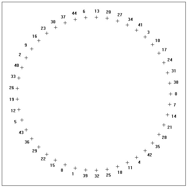
The figure shows how the unit circle forms piecewise starting at 0° and finishing at 44°.
45° would display at 0°; 46° would display at 1°.
The process would continue through 360° which is the complete circle.
Points on the unit circle stay on the unit circle when using polar coordinates.

There are infintely many degrees between each integer degree.
By addressing enough of these degrees, the circle would have no boundary gaps.

Note:
In this figure, the resultant θ points "wrap" after 0° through 44°; the entire 360° aren't shown.
The symbol "+" designates point value as single pixels are difficult to view.

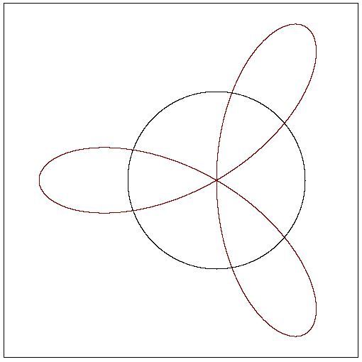
Polar Coordinate Unit Circle Variant with Pseudocode

for (int i = 0; i ≤ 180000; i++)
{
	x = 0.0;
	y = 0.0;
	θ = i*0.001;
	for (k = 1; k ≤ 2; k++)
	{
		θ = 2.0 * θ;
		xnew = cos(θ) + y;
		ynew = sin(θ) + x;
		x = xnew;
		y = ynew;
		if (k == 1) PlotPoint(x, y, black);
		if (k == 2) PlotPoint(x, y, red);
	}
}

Julia Polar	Build: (f(x,y,θ), g(x,y,θ))	Escape: k>value	Plot
Unit Circle	(cos(2^kθ), (sin(2^kθ))	k > 8	Point
Unit Circle Variant	(cos(2^kθ) + y, sin(2^kθ) + x)	k > 2	Point